The  Non-Mathematician's  Guide  To  Basic  Valveless  Pulsejet  Theory © 2008 Larry Cottrill                                                                   by Larry Cottrill   25 Sep 2008 Section 03.03.02 Putting On the Pressure Now we can get back to looking at things in a more conventional way, seeing the wave front as moving at Mach 1 speed through something resembling an engine pipe. What we want to see now is a magnified view of exactly how the changing pressure actually stirs air mass into motion. Let's re-cast the graphic we used above as the rather more complex drawing, below. 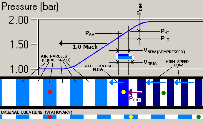Some explanation is needed of the added "features": The drawing is vertically divided into three zones; a large upper region showing the pressure wave graph, a crude representation of a length of straight pipe containing a row of adjoining air mass parcels as affected by the wave, and a narrow "ruler" mapping how the parcels were laid out before the arrival of the wave. The parcels in the pipe (and on the ruler) are alternately shown blue and white for clarity -- it must be kept in mind that whether a parcel is colored or white means absolutely nothing in terms of its behavior; they are all created equal, and assumed to all have exactly the same mass. A straight pipe (represented by the thick black bars) is used because it allows us to show changes in volume simply and precisely as changes in the thickness (i.e. length) of the parcels. Three of the parcels have been individually "marked" with colored dots; this is purely to clarify their motions, and has no other meaning -- they are exactly like all other parcels shown. A couple of final details: the drawing we used before showed the same parcel at two different moments in time; it was a kind of "before and after" shot. This graphic, on the other hand, shows all the adjoining parcels as they appear at a particular instant in time; a true "freeze frame" of the action. And, while the heavy black 1.0 Mach vector indicated the approach speed of air in the previous drawing, from now on it will indicate the speed of the wave front we're modeling: To see how pressure actually works to move air around, lets see from the picture above what happens to a particular air mass parcel. We'll choose the parcel "marked" with the yellow dot (shown in the "pipe" segment of the drawing). Each parcel of air has a finite length in the pipe; that is, it has a left face and a right face which adjoin neighboring parcels (the neighboring "white" parcels in the drawing). If we project the locations of these faces upward through the pressure wave front graph, we see that the left face cuts across a lower position on the pressure curve than the right face. We designate the height at which the left face crosses the curve as PLO and the height at which the right face crosses as PHI, representing two slightly different pressures. These are the actual static pressures on the two faces of the parcel, and they represent forces acting inward on it (because pressure x area = force). The relatively small pressure difference (PHI - PLO) is shown as PDIFF. I have brought PDIFF down into the pipe part of the drawing and shown it as a pressure vector acting on the yellow-dotted parcel. So, in effect, we see a net pressure (and therefore, a net force) acting as a leftward influence on the parcel. From elementary physics, we know that an object with a force acting on it accelerates in the direction the force is applied, and this is true of our selected parcel; I've tried to show this with the velocity vector labelled ACCELERATING FLOW -- the parcel indeed is moving leftward at increasing speed. The volume and density of the parcel are also affected by these pressures; however, it is a convenient and very close approximation to simply use the average pressure, which I have labelled PAV, as the effective pressure applied to the parcel as a whole. Note the little blue and white detail I've shown at about mid-height on the vertical projection lines. This shows how the volume (and length) of the parcel have been affected by applying pressure PAV. (Again, remember that because of the constant pipe cross-section, the volume of the parcel is perfectly represented by its length.) The original volume of the parcel is represented by VORIG and the modified volume by VNEW. The change in volume is inversely related to the change in pressure, so we can say that   VNEW / VORIG = 1.00 bar / PAV (since 1.00 bar was the original pressure) Again, I have used the darker blue color as a crude way of showing the higher density of the parcel due to its compressed state. As a mass of air is compressed, density essentially rises linearly with pressure. It should be remembered that the temperature of the parcel is increased somewhat by the compression, as well. But, unlike the relationship between pressure and density, the change in temperature is a highly non-linear function. From all of the above, we can formulate the following rule: The acceleration of a finite air mass comes from a force that is the result of a pressure difference. This pressure difference comes from the finite size of the mass and the non-uniform pressure represented by the wave front traversing the mass. Because "acceleration" is defined as a change in velocity (from basic physics), we can generalize the above (perhaps with some danger of oversimplification) as: CHANGES in air pressure cause corresponding CHANGES in air velocity. If we now move to the right side of the drawing, we find a region where the parcels in the pipe are highly compressed and are of perfectly uniform volume, density and temperature (that is, they are identical in terms of "local condition"). This can be seen to correspond to the flat top (or "plateau") of the pressure curve shown. The velocity vectors are given the label HIGH SPEED FLOW, and these vectors are exactly equal -- this is a region where the air speed is constant (i.e. no longer accelerating). As you may have guessed, it is no accident that constant speed flow corresponds to the constant pressure portion of the wave graph. In this part of the wave, the PHI, PLO and PAV are exactly equal, while PDIFF = 0. This means that, while pressure PAV still acts to compress each parcel, there is no longer any net force acting leftward on the parcels! Again looking at the situation in terms of basic physics, a mass with no net force acting on it keeps moving at unchanged velocity. That may seem counterintuitive if you have ever used compressor-powered air tools, or other high air pressure equipment -- after all, aren't you supplying pressure to maintain constant air flow through the hose to the tool? The real answer to that is, basically, no! What you are really doing is using compressor power to force the air up to its working pressure so the tool can recover that power at the other end. The movement of air through the hose would require NO power at all, if it weren't for friction losses in the hose and turbulence and shear losses in the fittings (and these effects account for only a tiny fraction of the total energy used). The actual motion of the air through the hose is essentially free. We should still note one more observation from the constant pressure / constant velocity region (the right end of the drawing): It is important to understand that the uniform air parcels in this region are not moving at the forward speed of the wave front. The forward speed of each parcel is basically determined by the compression of all those directly ahead of it!. Note the three "dotted" parcels shown in the pipe, then find the same three "dotted" parcels on the "ruler" below. Note that the "red-dotted" parcel is unmoved, the "yellow-dotted" parcel (being accelerated by increasing pressure) has moved a little, while the "green-dotted" parcel is already heavily displaced. Again, remember that this drawing is a "snapshot" of an instant in time; at this moment, the distances are closing between the "dotted" parcels, but in a moment the wave front will be completely past the "yellow" one, and the distance between it and the "green" one will then stay constant -- the "yellow" parcel will be at the velocity labelled HIGH SPEED FLOW. It is critically important that this concept be fully understood and accepted. So, what speed is our constant HIGH SPEED FLOW, anyway? We already have our answer, if we can measure the local air condition within the flat "plateau" part of the pressure wave (in other words, the condition after the front has completely passed by). From our previous discussion (where our viewpoint tracked right along with the wave), we observed that once a mass parcel of air has gotten to the final air condition region, it is traveling away from the front at a reduced speed we called UDEP; so, taking into account the actual speed of the wave front (1.0 Mach at the original condition, which is about 321.5 metres/sec), the actual reduced flow speed under the plateau of the curve (we'll call this speed UCondB) is easily derived: Duct Air Speed vs Condition B Pressure & Temperature   (Condition A = 1.0 bar air at 300 °K, stationary) PressCondB TempCondB 1.0 MachCondB UDEP UCondB MachCondB 1.1 bar 308 °K 325 m/sec 298 m/sec 24 m/sec .073 Mach 1.2 bar 316 °K 329 m/sec 276 m/sec 46 m/sec .139 Mach 1.3 bar 323 °K 332 m/sec 255 m/sec 67 m/sec .202 Mach 1.4 bar 330 °K 334 m/sec 237 m/sec 85 m/sec .254 Mach 1.5 bar 337 °K 337 m/sec 218 m/sec 103 m/sec .306 Mach 1.6 bar 343 °K 340 m/sec 202 m/sec 119 m/sec .352 Mach 1.7 bar 349 °K 342 m/sec 186 m/sec 136 m/sec .397 Mach 1.8 bar 355 °K 345 m/sec 169 m/sec 152 m/sec .442 Mach 1.9 bar 360 °K 347 m/sec 156 m/sec 166 m/sec .477 Mach 2.0 bar 366 °K 350 m/sec 141 m/sec 181 m/sec .517 Mach Warning: These values should be usable for areas of the pressure curve that are level (like the top of our our "plateau") or gradually changing (long smooth curves or slopes) -- they will not be accurate (and in many cases, not even close!) under rapidly changing zones of the wave such as pressure "spikes", or even within the "ramps" at the start and end of our "plateau" region! Fortunately, most of the time in pulsejets, the pressure is changing fairly gradually during the cycle. Again, we have assumed stationary air before the wave passes, i.e. UCondA = 0; in most real-life examples, we would not be starting with stationary air, but instead we would have some initial velocity at the region of interest in the pipe. This can be positive (in the same direction the wave front is moving) or negative (flowing against the advancing wave front) or (rarely) zero, as seen in our graphic example here. If non-zero, this initial velocity would simply be added algebraicly to the value in the table as selected for the local pressure. Thus, the flow velocity within the pressure wave can be readily determined even if all we know is the initial flow speed and the initial and final air conditions. When the actual speed for 1.0 Mach under any air condition is needed, it can be referenced in the table above (interpolating if necessary for greater accuracy). Go back to select another Section Next Section:   Letting Up